How to Save Millions by Self-Hosting LLMs
A practical guide to the economics of self-hosting open-weight LLMs. Using Kimi K2.6 and real production traffic from Cline, this post breaks down GPU memory, inference, batching, pricing, and the point at which self-hosting can save millions.

Preface
If you believe that cheap open weight models are the future then this blog is for you, we all know the why, but I will show you the how grounded in the economics behind it.
I wrote this because I can’t find this information in this form anywhere else. This is a single and arguably the only post that covers both the math of LLM inference and the dollars, grounded in production traffic and real numbers from inference provider negotiations.
If you find any errors in the math of this book, I will personally send you a printed copy of the book version and add you in credits section at the end.
Who is this for?
- Software engineers/Managers: shipping open-weight models
- AI research/Inference engineers: who want a working model of inference math + pricing
- Management Execs and PMs: wondering if self-hosting is worth it. You can skim the math, and read the dollar numbers at the end to decide.
- Students: chasing a job at a frontier lab
Prerequisites
All you need is high school algebra: every formula in this post is just multiplication, division, exponents etc. You don't need much ML background; transformers, MoE, KV cache, quantization, and everything else is either explained inline or linked to the best primer I could find. The blog is really dense, though, and the depth + understanding lives in the links. At a minimum budget a weekend if you want to actually internalize it.
What will we work with?
Our running example is Kimi K2.6, with Cline's real production traffic as the ground truth. The math works whether you rent your own GPUs or buy from an inference provider. We'll go in order: load the model, serve inference, batch it, and tune it for production.
Model Architecture
To self-host a model, you first load its weights onto a GPU. How much memory that takes is set by the model's architecture. Kimi K2.6 employs DeepSeek V3-inspired architecture with MoE parameters:
- Total parameters: 1 trillion (sparse MoE)
- Active Params: 32 billion
- Hidden size: 7,168
- Attention heads: 64
- Routed experts: 384
- Shared experts: 1
- Experts per token: 8
- MoE intermediate size: 2,048
- MoE layer frequency: 1
- Context window: 256K tokens
Want to derive these numbers from scratch? Read Kipply's legendary parameter counting post.
If you want some background on transformers architecture you must read: The Illustrated Transformer and if you are too tired to read another blog try LLM Visualizer which is the greatest LLM visualization I have ever seen.
Picking the GPU
We'll use the NVIDIA B200 (Blackwell). It's NVIDIA's flagship inference GPU and you can rent one from most neoclouds.
Here’s what you need to know about it:
- 192 GB HBM3e VRAM per GPU
- The standard HGX rack ships with 8 GPUs, wired together by NVLink. NVLink is a fast interconnect between GPUs, so the 8 GPUs can act like one big GPU during inference.
- Total GPU memory is 192 GB * 8 = 1,536 GB (~1.5 TB) per 8-GPU node
What does this node actually cost?
Let's lock in one number for the rest of the blog: $6 per GPU per hour. Real B200 pricing in 2026 is closer to $4 if you just rent the GPUS alone, but rounding up gives us a conservative ceiling, if the math works at $6, it will work in real life.
$6/GPU/hour × 8 GPUs        = $48 / node / hour
$48 × 24 hours              = $1,152 / node / day
$48 × 730 hours (avg month) = $35,040 / node / month
$48 × 8,760 hours           = $420,480 / node / year
That $48/hour is your fixed cost. Serving 1 user or 1,000, the meter runs the same. The rest of this blog is about squeezing as many tokens as possible out of that $48/hour as that's what sets your real $/token.
Note:
- Self-hosting only makes sense if you're already spending $35K+/month on API inference for this model. The model can't load on a smaller config, so $35K/month is the bare minimum entry ticket.
- You can rent just GPUs alone for as low as 3.5-4$ but if you work with inference providers they will charge you 5.5-6$ because they handle the hosting of the model/speculative decoding and all the other model serving magic. As you will later learn in this blog post paying for the extra money to get the models hosted by someone else is a VERY solid deal and much cheaper than hiring an inference engineer if you do it right.
How many GPUs do we need to load the model?
Figure out how big the weights are
Kimi K2.6 has 1 trillion params. We'll run it in FP4 quantization (0.5 bytes per param). Quantization basically means storing each weight in the model with fewer bits, like rounding $4.7283910 up to $5. The model gets way smaller in memory, and if done carefully, it gives almost the same answers.
FP4 is the aggressive quantization tier, and modern models are trained quantization aware, so the quality hit is not that bad, the models are easier to host, and far less memory is needed to load them on GPU.
weight_bytes = 1,000,000,000,000 × 0.5 byte = 500 GB
Divide by your GPU memory
500 GB ÷ 192 GB per B200 = 2.60
So 3 B200s technically fit the weights of FP4 quantized model. That's the floor and its enough to load the model into VRAM and nothing more.
Quantization and Quality
Quantization is a trade off between price and quality. On the pricing side, every number downstream of this section is linear in bytes-per-param. FP4 puts the weights at 500 GB; FP8 doubles that to 1 TB (you'd need 6 B200s, not 3); BF16 doubles it again. FP4 is the cheapest tier that still ships acceptable quality on modern quantization-aware models, which is why we use it. If your evals say FP4 hurts your workload, redo the chain at FP8 as the math still works, it just costs more. Note: FP4 here means NVFP4 specifically, Blackwell's native 4-bit format. And we'll use "FP4" throughout the blog for brevity.
On the quality side, the trade-off isn't visible on a spec sheet. Some providers offer dirt-cheap, low-latency inference but quantize so aggressively that output collapses no matter how good their latency SLAs(Service Level agreements) look. The only way to know what you're shipping is to run evals (our setup is here).
How many GPUs do we need to serve the model?
Loading the model is one thing. Serving real traffic is another, and it costs more VRAM. Every concurrent user needs their own slice of KV cache (per-user memory that keeps attention from being quadratic so that new inference requests use caching). You also need bandwidth and headroom to batch their requests efficiently. We'll cover KV Cache, bandwidth and headroom in the next sections, for now, just trust that this is where the rest of the VRAM goes.
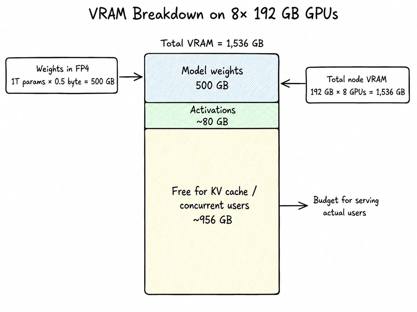
So we're taking the full 8-GPU B200 node: 1,536 GB of total VRAM. Here's how that breaks down:
| What | Math | Memory used | Remaining |
|---|---|---|---|
| Total VRAM on the node | 192 GB × 8 GPUs | — | 1,536 GB |
| Model weights | 1T params × 0.5 byte | 500 GB | 1,036 GB |
| Activations (working memory during a forward pass) | ~80 GB | 956 GB | |
| Free for KV cache (i.e. concurrent users) | ~956 GB |
That ~956 GB is the budget for actually serving users. The next several sections are how we spend it.
Serving the model
Two things happen on every request: the model reads the whole prompt (prefill), then writes tokens one by one (decode). We'll cover decode first because it's the dominant cost on long generations, then circle back to prefill.
Here's the TLDR of Decode. LLMs generate one token at a time. The model writes a token, looks at everything so far (your prompt + the tokens it just wrote), and writes the next one. It loops until its done.
[prompt] → token_1
[prompt + token_1] → token_2
[prompt + token_1 + token_2] → token_3
...
Each loop iteration is one forward pass: the input runs through dozens of layers, each layer reads its slice of weights from VRAM and hands its output to the next, and at the end you get a probability distribution over the next token. The model samples one and repeats.
So inference is just: read weights from VRAM → matrix math → emit a token → repeat.
Emitting a token (Decode)
For the 32B active params, if we have to generate an output token we need the following data flow(FP4 quantization is 0.5 bytes per param):
bytes_read_per_token = 32B active × 0.5 byte = 16 GB
16 GB of weight data flowing across the bandwidth pipe for every single token we generate. This is the main bottleneck number.
The B200 does 8 TB/s of memory bandwidth per GPU. Sounds enormous, but watch what happens when we run the math. Max output speed is just bandwidth ÷ bytes_per_token.
Single B200:       8 TB/s
8-GPU node (raw):  64 TB/s
8-GPU node (real): ~50 TB/s after sync overhead
50,000 GB/s ÷ 16 GB/token ≈ 3,125 tok/s theoretical
At 10–12% real-world MBU* ≈ 312–375 tok/s aggregate decode
So at small batch sizes, a full 8-GPU B200 node serving Kimi K2.6 in FP4 hits a theoretical ceiling of roughly 3,125 tokens per second of aggregate decode.
Decode is sequential so you can't generate token N+1 until token N is done. That's why decode is bandwidth-bound, and why TPS (tokens per second) is the metric that decides how fast the output streams. (Exception: speculative decoding.)
Caveats of theoretical max decode throughput vs actual max throughput
The 16 GB/token figure above assumes that every token reads its own personal slice of experts, which is true at batch=1, but it stops being true the moment you batch. Once many users flow through the same forward pass, tokens share expert reads inside MoE, the effective bytes-per-token shrinks, and aggregate decode climbs well past this number. There are also other aspects to consider. We'll work out exactly how this works in the Batching section.
That 3,125 tok/s number is theoretical: what you actually get is determined by your MBU (Memory Bandwidth Utilization), the fraction of nominal bandwidth your inference stack actually delivers to useful work. MBU varies widely: We measured ~11% MBU on vLLM + Kimi K2.6 + 8× B200 + 80K context, on the lower end.
Our practical takeaway is that you shouldn’t trust theoretical ceilings, and don't trust vendor claims either. You can do load tests and compute your achieved MBU as
(measured aggregate decode tok/s × bytes_per_token) ÷ nominal_node_bandwidth
Then cross-reference it with research papers to see if you are too far off, and if you are too far off then you must find out why.
Before going further, there's two ideas you need to lock in that will explain the real bottlenecks of GPU performance for inference and they are:
- Memory-bound vs compute-bound
- Arithmetic intensity
Memory Vs Compute bounds
This shows up constantly in transformer inference, and in deep learning optimization more broadly. The basic idea is that: to do any math on a GPU, you first have to pull the weights out of memory, which costs memory bandwidth. The good news (and this has been very well optimized) is that the GPU can start computing as soon as the first weights arrive memory reads and math run in parallel.
So at any given moment, one of two things is happening:
- Compute-bound/Flop-bound: In this case, the GPU is choking on math. The math units are fully busy, and memory is sitting idle. A FLOP is one floating-point operation. One multiply, one add, one of those. When people say a GPU does "15 PFLOPS," they mean it can do 15 × 10¹⁵ floating-point operations per second. You can read more about compute/flop bounds in these lecture notes.
- Memory-bound: the memory pipe is fully busy, and the math units are sitting idle.
Let me remind you once again that decode is memory-bandwidth-bound, and that is a huge bottleneck on how fast we can do our inference.
Arithmetic intensity
Since at any point the GPU is either memory or compute bound. Arithmetic intensity is the knob that flips a workload between the two: FLOPs done per byte read from memory.
arithmetic_intensity = FLOPs performed / bytes read from HBM
Every GPU has a break-even point (the "ridge" of the roofline model) where compute and bandwidth finish at the same time. Below the ridge you're memory-bound; above it you're compute-bound.
For the B200 at FP4:
ridge = peak_flops / peak_bandwidth
      = 10 PFLOPS / 8 TB/s
      ≈ 1,250 FLOPs per byte
So on a B200, a kernel needs to do ~1,250 ops per byte of weight before compute becomes the bottleneck. Anything less and the math units are sitting idle waiting on HBM.
Now look at where decode and prefill land:
- Decode (batch=1): ~2 FLOPs per byte read (one multiply-add per weight value). Deep in memory-bound territory. ~600× below the ridge. This is why decode tok/s is dictated by bandwidth, not flops(as i had mentioned before).
- Prefill: You read the same weight once and reuse it across thousands of tokens (or batching). Arithmetic intensity scales roughly linearly with how many tokens share that read. Push enough tokens through one forward pass and you cross the ridge into compute-bound land.
This is the lens to keep in your head for the rest of the blog. Every optimization that follows is, underneath, a trick to raise arithmetic intensity so each byte of HBM traffic produces more useful tokens. As we do load testing later and put more weight on our GPUs, we'll see both of these bounds in practice.
Loading the prompt tokens (Prefill)
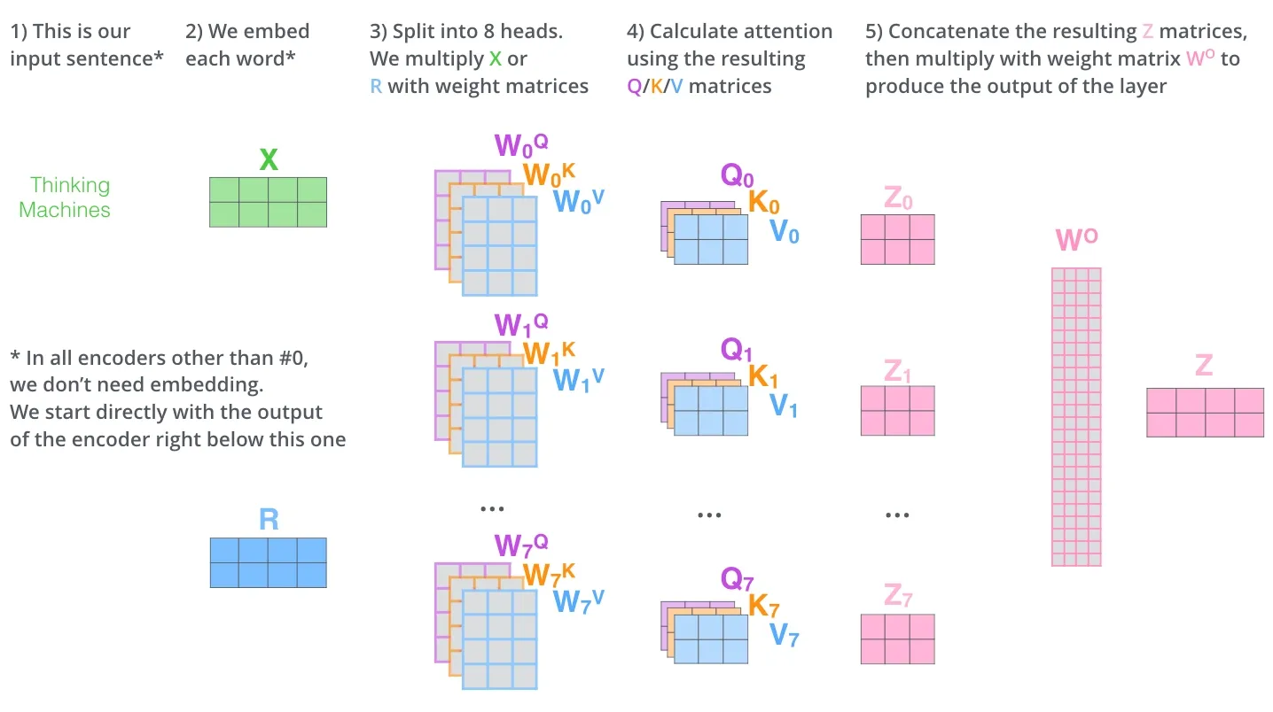
The next concept you need to learn is prefill. Prefill is when the whole prompt the user throws at you gets read in a large parallel mat mul operation so that the model can "process it" and give you a response (decode).
Why can you do prefill in parallel?
Because you already know the entire sequence, you can push it through the layers in parallel. In one weight read, thousands of tokens get processed simultaneously. The bandwidth bottleneck disappears because you're amortizing one read across thousands of tokens.
Prefill is compute-bound. In our case, the B200 GPU has way more compute than bandwidth: ~10 PFLOPS dense at FP4 per GPU, and we have 8 GPUs.
Realistic prefill speeds reach ~78,000 input tokens/sec aggregate on an 8-GPU B200 node, roughly 1 coding-agent-sized fresh prompt processed per second on a long Kimi K2.6 conversation. That's what we'd expect to measure at Cline running this workload.
Math to explain it
Flops per GPU    = 10 PFLOPS
flops_per_token  = 2 × 32B active = 64 GFLOPs
node_compute     = 8 GPUs × 10 PFLOPS = 80 PFLOPS (dense FP4)
theoretical_max  = 80 PFLOPS ÷ 64 GFLOPs ≈ 1.25M tok/s
realistic        ≈ 6.4% MFU (attention quadratic + MoE all-to-all,
                          partially offset by B200 attention pipeline)
                 ≈ 78,000 tok/s on long prompts (this was what we got in load testing)
MFU(Model FLOPS Utilization) = (achieved FLOPs/sec on model work) / (peak FLOPs/sec of the hardware)
MFU is the reality check on your prefill numbers. Compare your measured MFU against the ranges published in literature if you're too far off, either your stack has a real problem or another provider is squeezing far more out of the same hardware.
TTFT: Time To First Token
This is where the metric TTFT (Time To First Token) comes from, the wait between hitting enter on chat and seeing the first character stream back. Everything before the first token appearing on chat is prefill burning compute. Everything after is decode burning memory bandwidth.
If your node prefills at 80,000 tok/s and a user shows up with an 80,000-token prompt:
80,000 tokens ÷ 80,000 tokens/sec = 1 second TTFT
In practice, two things change this number by a lot in different directions:
1. Batching: That 80K tok/s is the whole node of the entire GPU. If 16 users are prefilling concurrently, each one only gets ~5,000 tok/s of effective throughput. An 80K prompt now takes ~16 seconds. Per-stream and aggregate are very different numbers, and you need load tests in different configurations to figure this out. We will explain batching more later in this document.
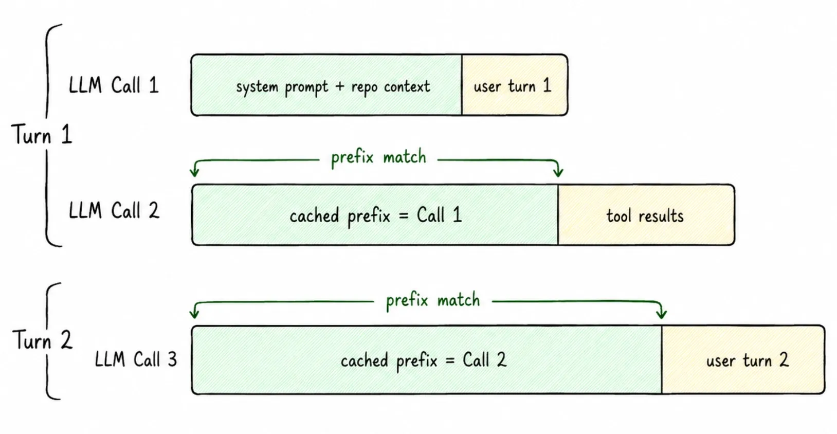
2. KV cache/Prompt reuse: In coding agents and chat, conversations build on top of each other. When a user fires off their 5th message in a long thread, you're not re-prefilling the entire 80K context the KV cache from earlier turns is already sitting in VRAM. You only prefill the delta: the new user message plus whatever fresh context got pulled in (file reads, tool outputs, etc).
At Cline, our system prompt is small, roughly 3–4K tokens, and most of the tokens come from file reads/searches over the back-and-forth conversation. Even when total context is 80K, the actual new tokens being prefilled on a given turn are usually 8–10K, mostly from file reads.
KV Cache: where the 956 GB actually goes
Remember that ~956 GB of free VRAM we left in the bank earlier? This is where we spend it.
Here's the core problem KV cache solves. Every time the model decodes a new token, the attention layer needs the K (key) and V (value) vectors of every previous token in the context. Without caching, you'd recompute every K and V from scratch on every single decode step, turning each new token into a fresh prefill of the entire history. That's quadratic work for nothing.
The fix is simple: K and V from past tokens are deterministic functions of those tokens, and the model weights don't change. So the K and V you compute at step 5 are literally the same numbers you'd compute again at step 6, step 7, step 10. Compute once, keep in VRAM, read back on every future step.
The picture above is the main intuition.
Insight 2: the next token's attention only needs the new token's query vector and all past key/value vectors. New Q every step, but the Ks and Vs from prior steps are reusable forever.
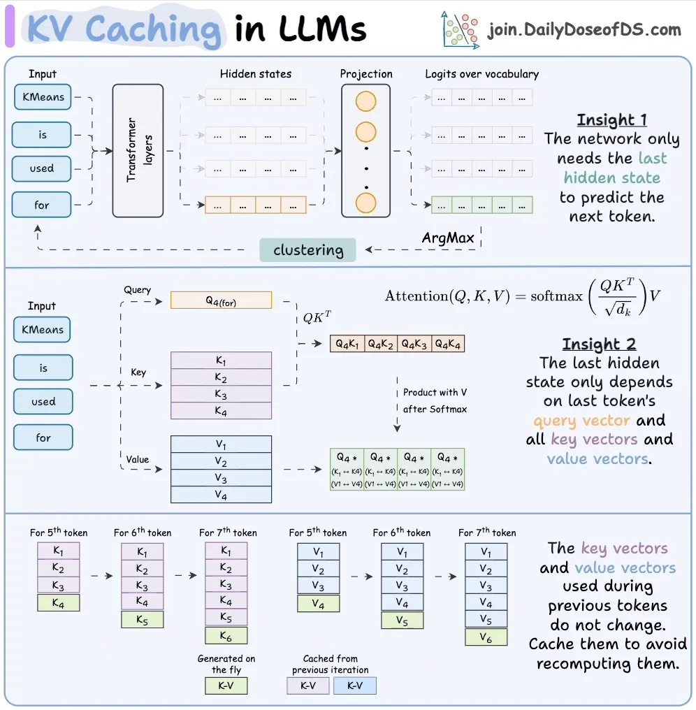
So the cache works like this: on token 5, you generate K_5 and V_5 fresh and append them to the K/V buffers. Tokens 1–4 get pulled from cache. On token 6, you append K_6 and V_6 and pull tokens 1–5 from cache. One new pair per step, never recomputed. That's the whole game.
How big is the cache, in bytes?
DeepSeek V3 and Kimi, which inherits the attention architecture, use MLA: Multi-head Latent Attention. Instead of caching K and V for every head, MLA compresses them into a single shared latent vector per layer plus a small RoPE component. The cache size becomes independent of head count.
bytes_per_token (MLA) = num_layers × (kv_lora_rank + qk_rope_head_dim) × bytes_per_value
                      = 61 × (512 + 64) × 1
                      ≈ 35 KB / token / user
Caching in the 956 GB
KV per user = 35 KB × context_length. Free VRAM = 956 GB. So:
max_users ≈ 956 GB / (context_length × 35 KB)
| Context length | KV per user | Theoretical max users |
|---|---|---|
| 80K (Cline-shaped) | 2.80 GB | ~341 |
| 32K (typical chat) | 1.12 GB | ~853 |
This is the theoretical ceiling, but not the operational ceiling. All of this would only be true if we assume that the entire remaining VRAM was just used for KV cache but the truth is far more complex. We can't actually support 341 users at the same time(we can barely support 32). Now let’s figure the why out in the batching section up next.
Batching
The whole point of batching is that decode is memory-bandwidth-bound. At batch size=1, you pay the full cost of pulling weights from HBM just to generate a single token for a single user. That's wasteful, the weights are already on the wire, you may as well pipe more tokens.
So you stack many users' next-token computations into the same forward pass. Each pass reads the model weights once, and every user in the batch shares that read. If you can fit B users into a pass, you get B tokens out for roughly the cost of one read. That's the main trick.
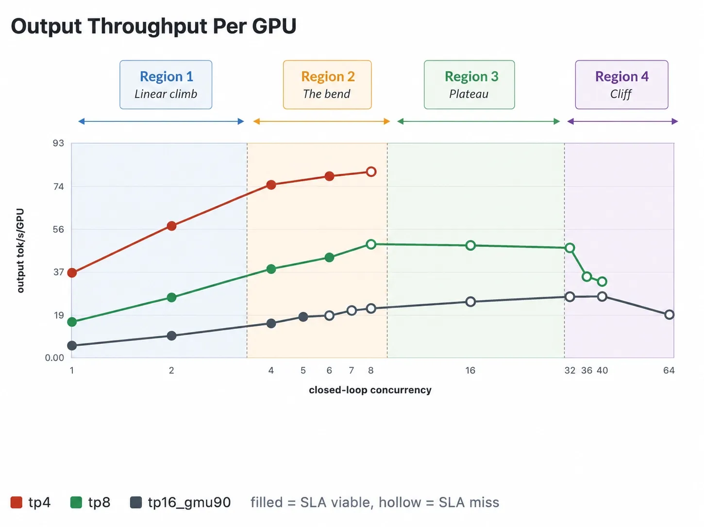
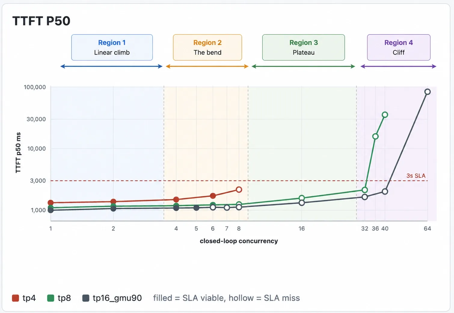
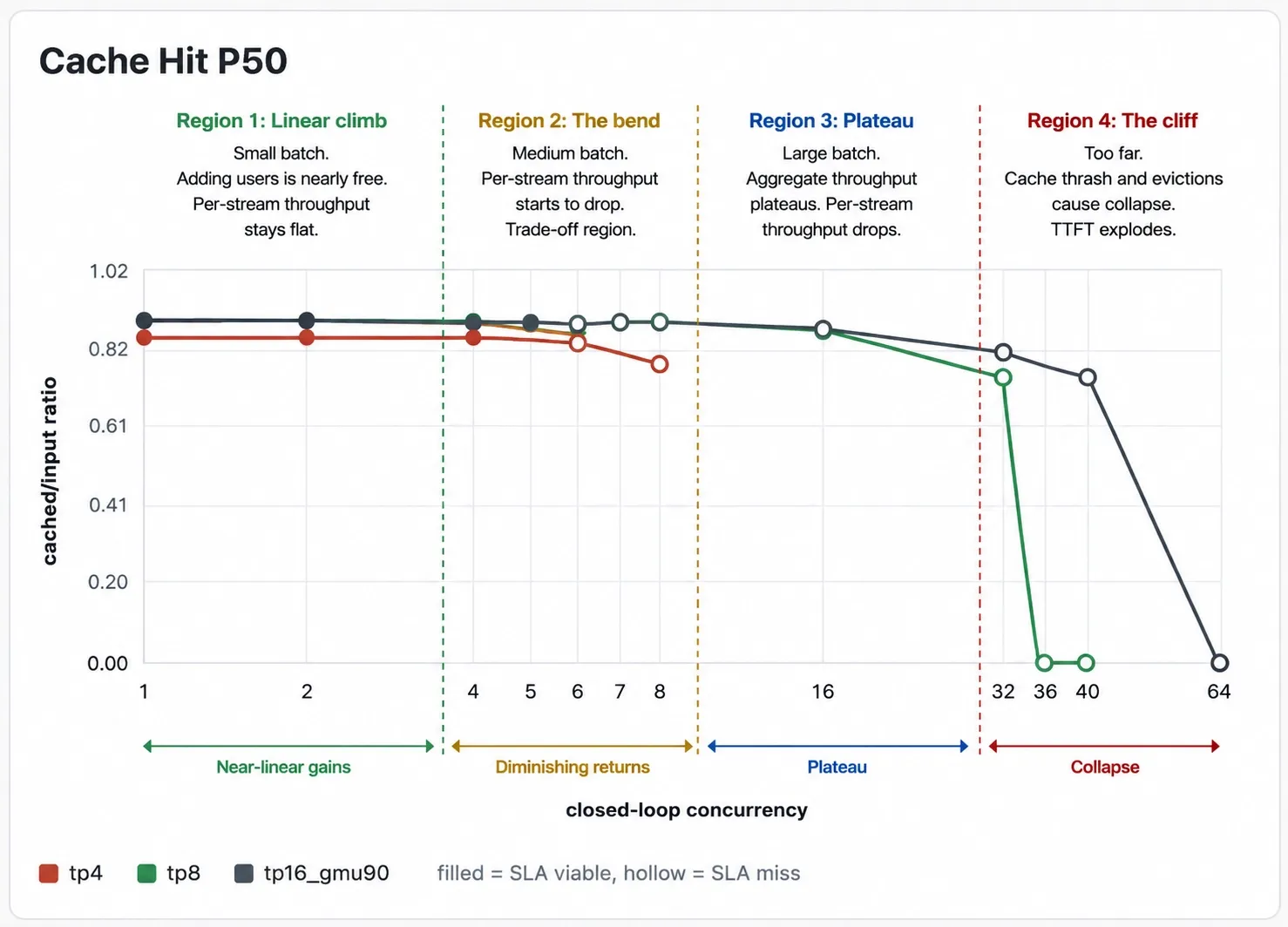
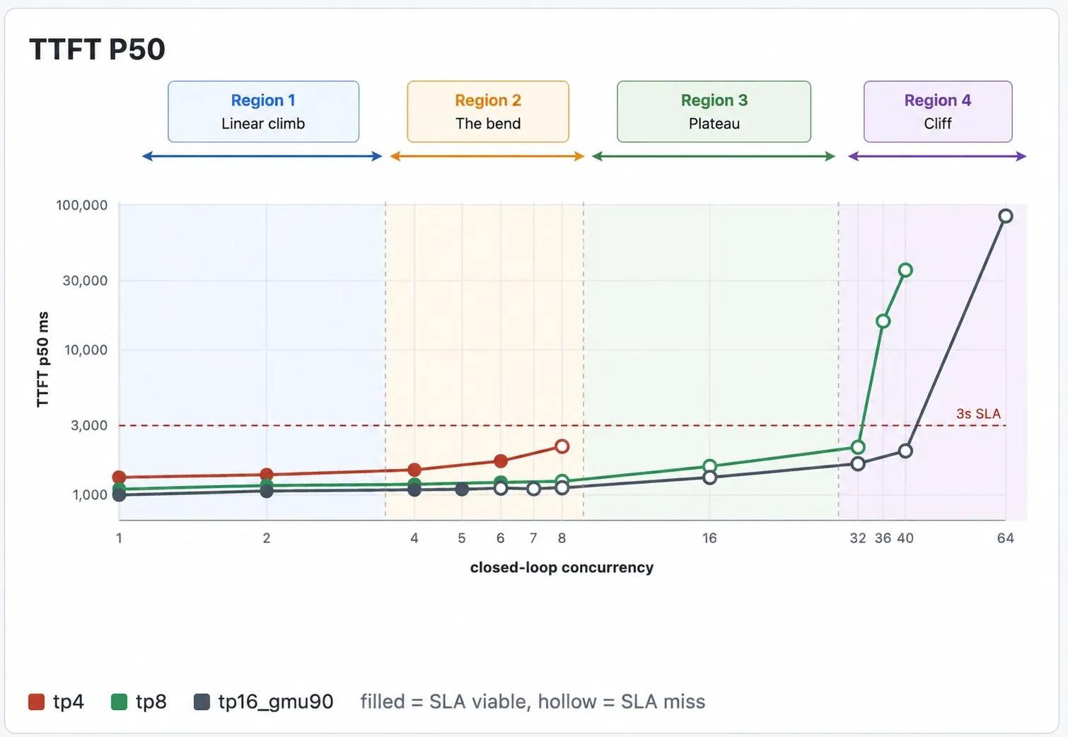
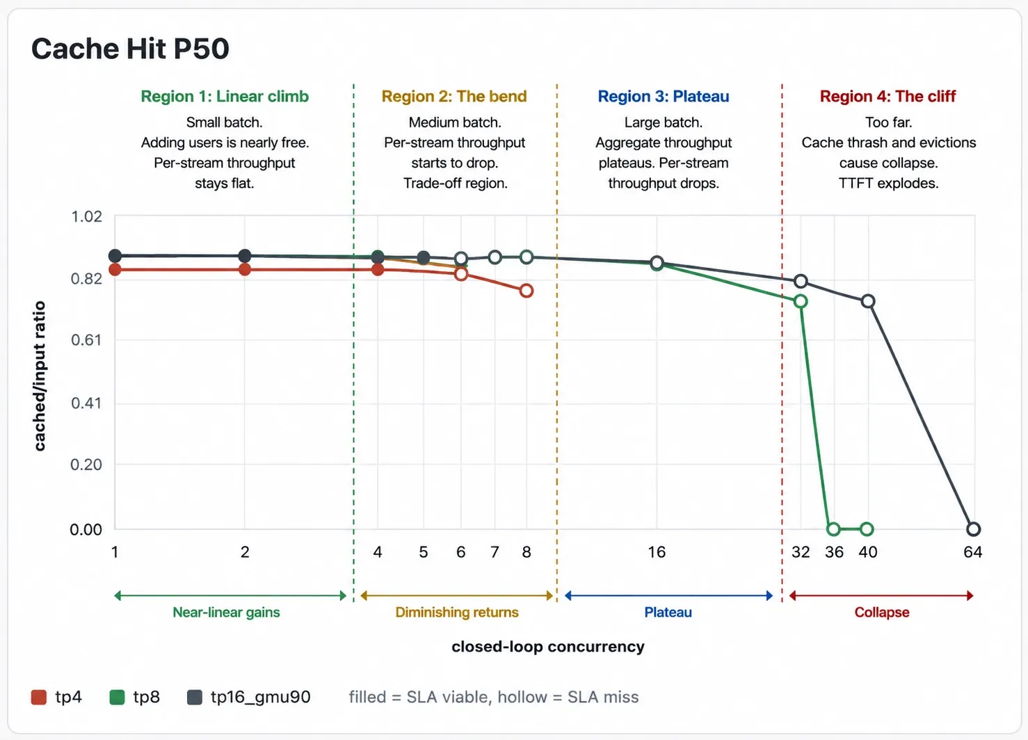
But the savings have their own limitations, and the curve of "what happens as B grows" is an important shape in inference economics. It plays out in four regions, with clean bends between them.
Region 1: The linear climb (small batch)
At low batch sizes, every additional user is nearly free. You're memory bound, and the GPU has tons of compute headroom sitting idle. Adding another stream to the pass costs you almost nothing on the bandwidth side because:
- Shared weights (attention layers, embeddings, the always-on shared expert) are read once per pass, regardless of how many users you stack into it.
- KV cache reads do scale linearly with batch (each stream has its own context), but at small batches their bytes are dwarfed by the weight reads.
So in this region, aggregate throughput climbs almost linearly with batch size, and per-stream throughput stays flat. Adding users is a pure efficiency win, the same bandwidth bill has more tokens per second out the door. Each user still sees the same fast stream even though we are scaling up concurrency.
Region 2: The bend (medium batch)
Eventually batch grows large enough that the dynamics shift. Two things happen at once:
- KV cache reads pile up linearly. Each conversation stream pulls its own context's worth of K/V on every decode step, and at long context that's a fat number. Once KV reads become a meaningful fraction of per-pass bytes, scaling stream count scales bandwidth demand 1-to-1.
- Attention compute climbs with batch. The math is roughly: For each user in the batch: take their current token's Q vector, dot-product it against their entire context of K vectors, softmax, weighted-sum their V vectors. Obviously, it's not amortized across users the way weights are and therefore the compute grows with batch size.
The combined effect is that aggregate throughput bends downward off the linear line, and per-stream throughput starts dropping noticeably. You're still adding users productively, but each one costs more than the last and slows everyone else down a little.
This region is where you have to make a real decision of how much per-stream latency are you willing to trade for more concurrent users? The answer totally depends on your SLA as coding agents and chat etc have very different tolerances.
Region 3: The plateau (large batch)
Push batch further and you hit the floor. What's left is per-stream cost: KV reads, attention compute.
- These all grow linearly with batch, with no sharing left to exploit. The bottleneck doesn't change you're still memory-bound but the bandwidth is now spent on per-stream KV reads instead of shared weight reads, and there's nothing left to amortize.
Pushing past this point is actively counter-productive. You're slowing every user down for no aggregate gain.
Region 4: The cliff (too far)
There's one more region past the plateau, and it's the worst one. KV cache memory is finite. Each additional concurrent stream needs its own slice of VRAM to hold its context's K/V. Push concurrency high enough and the working set exceeds free VRAM, the engine starts evicting cached prefixes to make room, returning users miss cache and have to re-prefill from scratch, that stretches every request, which holds VRAM longer, which forces more eviction.
This is a positive-feedback collapse. Aggregate here falls off a cliff, and TTFT explodes from seconds to tens of seconds. The operational rule is to never run a node where working set is anywhere near the VRAM ceiling.
Putting the regions together
| Region | What's happening | Aggregate TPS | Per-stream TPS | Bottleneck |
|---|---|---|---|---|
| Small batch | Shared weights amortize cleanly, KV is small | climbs ~linearly | flat | HBM bandwidth |
| Medium batch (the bend) | KV and attention compute start dominating | bends sub-linear | starts dropping | KV reads + attention compute |
| Large batch (the plateau) | No more amortization left, every byte is per-stream | flat | crashes | HBM bandwidth (per-stream KV) |
| Cliff | Working set exceeds VRAM, eviction cascade | collapses | unusable | KV cache memory |
How to pick the right batch size for your config
After all this, you probably want to know which batch size is best for your workload and sadly, there's no single answer. Coding agents, chatbots, agentic loops, and bulk generation each land in a different spot on the curve.
As an operator, your job is to find the largest batch size that still meets the per-stream SLA. Smaller leaves money on the table, and larger drops users below the SLA threshold for no aggregate gain. The goal of cost economics is figuring out which side of the bend your workload sits on and what works specifically for you.
Very often, you can't just grab a config online and ship it. vLLM and others publish reference configs, but those are tuned to specific traffic shapes and if yours differs, you can’t do the plug and play.
You need to load test to figure this out. Think of it as a search problem where you're searching the configuration space for the point that gives you the best value, and the only way to evaluate a point is to run your real traffic through it and measure what happens.
I'll talk more about working with inference providers and load tests later, but for now let me walk you through a load test we ran that helped us figure out the performance on different batch sizes and GPU configurations.
Load test config
Our load test was done by the kind folks at CoreWeave. We tested TP4, TP8, and TP16 with batch sizes of 1, 2, 4, 8, 16, 32, 64 to figure out what works best for us.
We could walk through every batch size from 1 to 64, but the curve does exactly what theory predicted linear climb, bend, plateau, cliff and the only point that matters for cost economics is the plateau: the batch size where aggregate throughput is maximized before per-stream speed collapses.
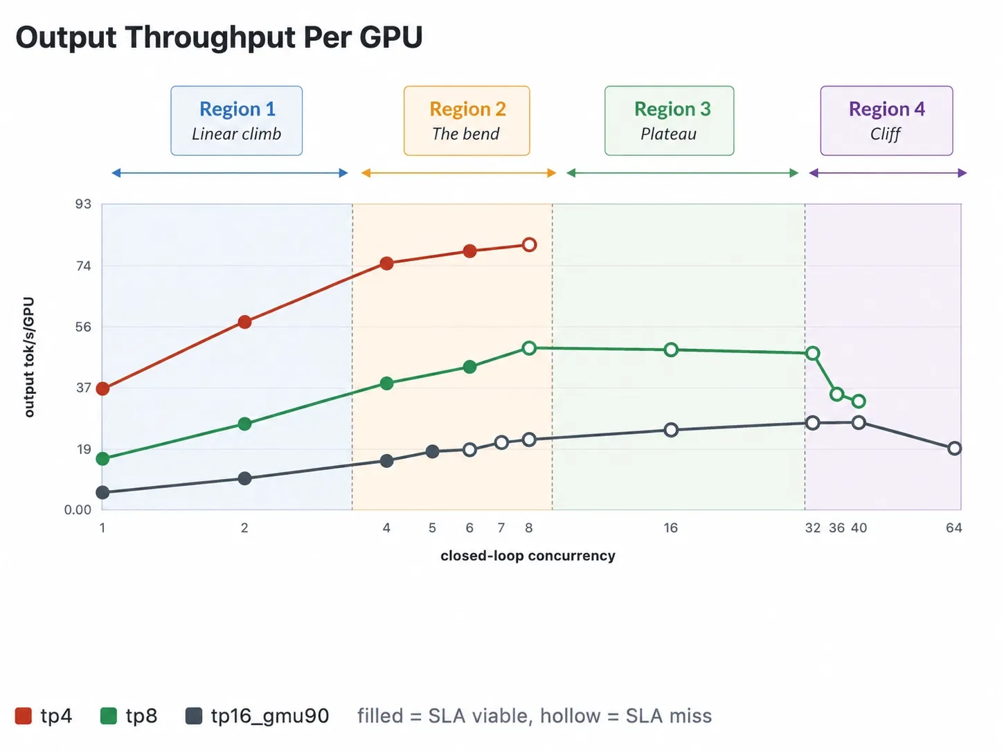
For TP8 + Kimi K2.6 on Cline's workload, that's batch size = 16.
Why B=16 over the other obvious candidates:
- B=8 is faster per stream (~54 tok/s), but the node is under-loaded, aggregate hasn't hit the bandwidth ceiling yet.
- B=16 sits exactly at the throughput plateau. Peak aggregate output, lowest $/token, cache hit rate still healthy.
- B=32 keeps aggregate flat (no improvement over B=16) but per-stream collapses to ~14 tok/s. Same total tokens out but much worse per-user latency.
- B=36+ is past the cache cliff. TTFT explodes, cache effectiveness collapses, throughput crashes.
Napkin math breakdown of a single config
We're only showing the math for one batch, B=16, because that was the operating point where we observed the highest utilization without exhausting the cache. There's a separate question we're parking until after this walkthrough: whether running 8 GPUs as one tensor-parallel group is even the right structure: we tested TP4, TP8, and TP16 configs. We'll come back to it once the per-batch math is anchored, because that answer matters more than batch size does.
With this breakdown, you'll get critical SLA values like tokens per second, aggregate output tokens per second, processed throughput per node, cost per million processed tokens, and time to first token. We'll derive each one from first-principles math, then confirm it matches the load test. You should do this exercise for your own config.
Formula chain
For any batch size B, decode throughput falls out of five steps:
per_pass_bytes(B)   = routed expert reads + shared/dense weights + KV reads
memory_time(B)      = per_pass_bytes / (bandwidth × MBU)
per_pass_time(B)    = fixed_overhead + memory_time × overlap_factor
per_stream_TPS(B)   = 1 / per_pass_time
aggregate_TPS(B)    = B × per_stream_TPS
Hardware constants for the 8× B200 node:
- Effective HBM bandwidth: 50 TB/s (raw 64 minus sync overhead)
- Effective MBU on MoE long-context: real-world vLLM/MoE typically lands closer to ~11% as measured above
- Fixed per-pass overhead (TP collectives + MoE all-to-all + kernel launches): ~5.2 ms (linear-fit intercept from measured 8-GPU benchmarks)
Case: Batch = 16
Step 1: Bytes per pass:
| Component | Math | Bytes |
|---|---|---|
| Routed experts hit | ~109 unique experts/layer × 61 × 22.5 MB | ~149 GB |
| Shared weights (attention + embeddings + shared expert) | constant | 5.6 GB |
| KV cache reads (80K context) | 16 × 2.8 GB | 44.8 GB |
| Total per pass | ~200 GB |
The 109 unique experts come from 384 × (1 − (376/384)^16) ≈ 109.
Naively 16 tokens × 8 experts/token = 128 expert slots, but only ~109 are unique, the rest are duplicates picked by multiple tokens. That's the sub-linear expert sharing(See Occupancy problem).
Step 2: Memory time (napkin math):
memory_time = 200 GB / (50 TB/s × 0.50 MBU)
            = 200 GB / 25 TB/s
            ≈ 8.0 ms
We take a 50% MBU assumption here.
Step 3: Per-pass time:
Per-pass time is how long one decode forward pass takes, the time the GPU needs to read all the weights + KV for the batch, do the math, and emit one new token to each user in the batch.
Measured in load test: ~36.8 ms at B=16. The number actually worth using as a predictor is the empirical linear fit from our 8-GPU benchmarks. We got the linear fit by making a linear equation from the TPS and Per pass times of benchmarks at different config to get a per pass time equation as a function of batch size:
per_pass_time(B) ≈ 5.2 ms + 1.65 × B
per_pass_time(16) ≈ 31.6 ms   (~14% off measurement)
The remaining ~14% on top of the fit is attention compute, which starts to bite past B=8.
For contrast, here's what the first-principles napkin from Step 2 predicts:
napkin per_pass_time = 5.2 ms fixed + 8.0 ms × 0.5 overlap
                    ≈ 9.2 ms
That's 4× off measurement, and it's worth pausing on why. The napkin smuggles in two optimistic fudge factors: a 50% MBU assumption ( in reality its is closer to 13% on vLLM + MoE + 80K context) and a handwavey overlap factor. Each one is off by roughly 2×; compounded, they account for the full 4× gap.
Later in the blog we have Warnings for engineers section which mentions that first-principles napkins routinely miss real inference stacks by 2–10×. I am not saying don't do napkin math, I am saying that you could use napkin as a sanity check but use the empirical fit as the predictor, and always carry both.
Step 4: Per-stream TPS:
Per-stream TPS = 1 / per_pass_time
per_stream_TPS = 1 / 0.0368 sec ≈ 27 tok/s per user
27 tok/s per stream is acceptable for our use case, it's roughly the speed you'd get from OpenRouter for this model anyway, so users won't notice. Note that: this was the observed value as well.
Step 5: Aggregate output TPS:
aggregate_output = output_per_GPU × 8 GPUs = 48.7 × 8 ≈ 390 tok/s
We compute this directly from the measured output throughput per GPU times 8, rather than the naive B × per_stream_TPS = 432, which overcounts because it ignores TTFT and end-to-end occupancy time.
Step 6: Total processed throughput per node (Little's Law):
For Cline's load test traffic, an average request looks like:
fresh tokens (avg):   ~13K   (new content per turn,  ~16.5% of input)
cached tokens (avg):  ~71K   (prefix from KV cache,  ~83.5% of input)
output tokens (avg):  ~1K    (typical coding-agent response)
proc tokens/request:  ~85K   (fresh + cached + output)
To turn per-request tokens into per-second throughput, use Little's Law: in a steady-state system, throughput equals concurrency divided by end-to-end latency per item.
To get processed throughput:
per-stream TPS (lifecycle) = 390 / 16        ≈ 24 tok/s
e2e per request           ≈ 1,000 / 24       ≈ 41.8 s
sustained req/s           = 16 / 41.8        ≈ 0.38 req/s per node
proc throughput           = 0.38 × 85K       ≈ 32K proc tok/s per node
To get end-to-end latency:
decode_time = output_tokens × per_pass_time
            = 1,056 × 36.8 ms
            ≈ 38.9 seconds

e2e ≈ TTFT + decode_time
    ≈ 1.6s + 38.9s
    ≈ 40.5 seconds   (measured: 41.84s, within 3%)
Two things to call out about that chain:
- The per-stream number is the lifecycle TPS from Step 5 (390 ÷ 16), not the 27 tok/s steady-state decode rate from Step 4. The lifecycle number already bakes in the prefill tax, so we don't need to add TTFT separately.
- The 83.5% cache hit rate doesn't change
proc tok/sinput counts as processed whether it's cached or fresh. The cache split matters in two other places: (a) Step 8's TTFT math, where only the fresh portion drives prefill load, and (b) API pricing, where cached input bills at a discount.
Sanity check against Step 5: the output share of that 32K is 0.38 × 1K ≈ 380 tok/s, which reconciles with the 390 tok/s aggregate output from Step 5 within rounding. Checks out.
Step 6: Total processed throughput per node (Little's Law):
For Cline's load test traffic, an average request looks like:
fresh tokens (avg):   ~13K   (new content per turn,  ~16.5% of input)
cached tokens (avg):  ~71K   (prefix from KV cache,  ~83.5% of input)
output tokens (avg):  ~1K    (typical coding-agent response)
proc tokens/request:  ~85K   (fresh + cached + output)
To turn per-request tokens into per-second throughput, use Little's Law: in a steady-state system, throughput equals concurrency divided by end-to-end latency per item.
To get processed throughput:
per-stream TPS (lifecycle) = 390 / 16        ≈ 24 tok/s
e2e per request           ≈ 1,000 / 24       ≈ 41.8 s
sustained req/s           = 16 / 41.8        ≈ 0.38 req/s per node
proc throughput           = 0.38 × 85K       ≈ 32K proc tok/s per node
To get end-to-end latency:
decode_time = output_tokens × per_pass_time
            = 1,056 × 36.8 ms
            ≈ 38.9 seconds

e2e ≈ TTFT + decode_time
    ≈ 1.6s + 38.9s
    ≈ 40.5 seconds   (measured: 41.84s, within 3%)
Two things to call out about that chain:
- The per-stream number is the lifecycle TPS from Step 5 (390 ÷ 16), not the 27 tok/s steady-state decode rate from Step 4. The lifecycle number already bakes in the prefill tax, so we don't need to add TTFT separately.
- The 83.5% cache hit rate doesn't change
proc tok/sinput counts as processed whether it's cached or fresh. The cache split matters in two other places: (a) Step 8's TTFT math, where only the fresh portion drives prefill load, and (b) API pricing, where cached input bills at a discount.
Sanity check against Step 5: the output share of that 32K is 0.38 × 1K ≈ 380 tok/s, which reconciles with the 390 tok/s aggregate output from Step 5 within rounding. Checks out.
Step 7: Cost per million processed tokens:
node_cost          = $48 / hour
proc_throughput    = 32K tok/s × 3,600 = 115M proc tok/hour
$/M processed      = $48 ÷ 115M  ≈  $0.42 / M
In other words, if the GPU is running flat out around the clock, every million tokens processed through it costs us $0.42.
Step 8: TTFT (time to first token):
The same chain also predicts TTFT, which is set by how long it takes to prefill a new request's fresh tokens while sharing compute with the other concurrent users in flight:
TTFT ≈ fresh_tokens × concurrency / replica_prefill_rate
At TP8 c=16 with Cline's workload:
fresh_tokens (median):       ~9,400 tok/request
replica_prefill_rate:        ~78,000 tok/s  (8× B200, ∼6.4% MFU)
concurrency:                 16
TTFT ≈ 9,400 × 16 / 78,000  ≈  1.9 seconds
The measured TP8 c=16 TTFT p50 was 1.57s during our load tests: the napkin matches the measurement within ~20%.
Notice how we calculated most of the critical SLA values here, both from first principles and then also verified them from the load test. This is the point of doing it in napkin math so that you can see how the puzzle pieces of inference optimization fit together.
What we actually used: TP4 c=8
This example of TP8, C 32 (8 GPUs per replica, 32 concurrent users per replica) is a great for explaining the inference math but not so much for prod work loads. The $0.42/M number is proper pricing math, but the comparison with the API ($0.317/M) does not justify the operational complexity of running our own inference.
The perfect value we actually used was TP4 c=8 (4 GPUs per replica, 8 concurrent users per replica), and the dollar math gets meaningfully better.
The same formula chain at TP4 c=8 gives:
GPUs per replica:        4
Cost per replica/month:  4 × $6 × 730 = $17,520
Per-stream TPS:          ~46 tok/s
Per-replica proc tok/s:  ~26,600
Tokens per replica/mo:   26.6K × 3600 × 730 = 70 B at 100% utilization
$/M processed:           $17,520 ÷ 70,000 = $0.250 / M
Two TP4 replicas fit on each 8-GPU physical node, so the same $48/hr box now produces ~53K proc tok/s instead of 32K, so the same hardware has ~63% more throughput. This was because smaller tensor-parallel groups (4 GPUs vs 8) have less cross-GPU sync overhead per forward pass, which more than offsets the smaller batch per replica. At TP4 c=8, self-host is ~21% cheaper than the API per token, but only if the replicas stay busy all the time.
Sizing the fleet of GPUs
Self hosting has fixed cost. The problem with GPUs is that a box that's 50% idle effectively doubles its $/M token. So we don't size for peak load, we size for the floor of the load, the lowest hour of the day, so the boxes stay at 100% utilization 24/7. Everything above the floor flows to the API via LiteLLM and this way we maximize GPU usage.
Cline's traffic shape (from three days of our gateway data):
| Scenario | QPS | Concurrent (in-flight) | Total proc tok/s |
|---|---|---|---|
| P50 (median hour) | 2.6 | 73 | ~222K |
| P90 (busy hour) | 3.4 | 103 | ~290K |
| P99 (peak hour) | 3.8 | 111 | ~327K |
| Estimated trough (overnight) | — | — | ~110K |
To keep all replicas at 100% utilization, we size at ~the trough:
N replicas × 26.6K proc tok/s ≤ 110K proc tok/s
N ≤ 4 replicas (= 2 physical 8-GPU boxes)
4 TP4 replicas (2 physical boxes) is the largest fleet that runs 100% utilized 24/7. Everything above flows to the API via LiteLLM.
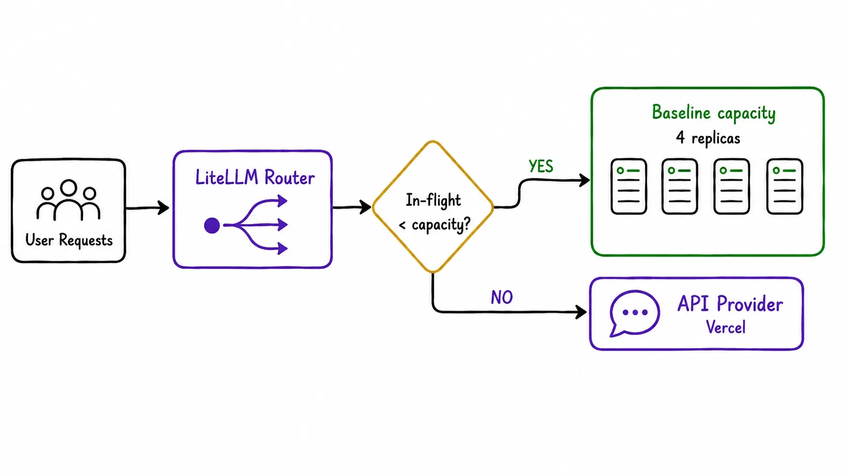
Self-host (4 TP4 replicas, 100% utilized):
  Cost:            4 × $17,520 = $70,080 / month
  Tokens served:   4 × 70B = 280 B proc tokens / month

API spillover (everything above 4 replicas):
  Tokens served:   583B − 280B = 303 B proc tokens / month
  Cost:            303B × $0.317/M = $96,051 / month

Total:             $70K + $96K = $166K / month
The monthly bill
Comparison to pure API
All API:                  583B × $0.317/M = $185K / month
Self-host + spillover:    $166K / month
Net discount:             $19K / month (~10% savings)
About 10% savings vs. pure API, with zero operational risk: if the self-host fleet has issues, the API picks up everything above the trough automatically. The discount comes entirely from running 4 replicas at $0.250/M continuously instead of paying $0.317/M for those same tokens at the API. The discount could have been bigger, We're leaving money on the table. The $96K/month going to API spillover is the expensive bucket, every token through it costs $0.317/M instead of $0.250/M. If we autoscaled additional self-host capacity during the predictable peak hours (matching the daily peak/trough pattern instead of sitting at the floor 24/7), we could shift a lot of that spillover onto the cheaper self-host rate.
The possibilities of financial savings
Rough estimate: time of day autoscaling could push total savings to 22–25% (closer to $40–50K/month). It's the next optimization on the list(not yet implemented). There are other optimizations and load tests of different cases which weren't explored as deeply. And had they been explored and more cases been tried, it's very plausible that our discount could even easily go to 35 to 40% on the API pricing.
| Monthly API spend | Annual API spend | Baseline self-host savings (floor-sized fleet, like Cline's deploy) | With time-of-day autoscaling | Aggressive (extra GPU tricks + relaxed SLAs) | Annual $ saved at best case |
|---|---|---|---|---|---|
| < $35K | < $420K | impossible (one 8-GPU box is the minimum unit) | — | — | — |
| $35K – $100K | $420K – $1.2M | marginal, not worth ops cost | ~5–10% | ~10–15% | up to ~$180K/yr |
| $100K – $500K | $1.2M – $6M | ~10–15% (Cline's zone) | ~20–25% | ~30–35% | up to ~$2.1M/yr |
| $500K – $2M | $6M – $24M | ~15–20% | ~25–30% | ~35–40% | up to ~$9.6M/yr |
| $2M+ | $24M+ | ~20%+ | ~30%+ | 40%+ (custom kernels, speculative decoding, batch tuning, loose latency SLAs) | $10M+/yr |
A few things worth saying out loud about this table:
- The floor-sized column is what you get with the no-risk deploy we described above: size the fleet to the trough of daily traffic, run those replicas 100% utilized 24/7, and let LiteLLM spill everything else to the API. This is the column you should plan against if you're shipping this next quarter.
- The autoscaling column assumes you match the daily peak/trough shape: more replicas during business hours, fewer overnight. The savings jump because you're now serving the expensive spillover bucket on the cheaper self-host rate instead of the API.
- The aggressive column is what's reachable if you're willing to spend real engineering effort: tighter MoE kernels, speculative decoding tuned to your workload, quantization-aware evals to push to FP4 (or lower) without quality regression, batch-size hunting per workload class, and accepting slightly looser per-stream TPS SLAs for back-of-the-pipeline traffic (bulk, async, agentic loops).
- At $2M+/month of API spend ($24M+/yr), the absolute dollar savings start running into eight figures annually. At that scale, the ops cost of running your own inference stack stops being the question, the question becomes how fast you can hire the team to chase the next 5% MFU.
Self-hosting vs. inference providers
You can actually self-host. The math in this blog is enough to get you started. But for most teams, I'd strongly advise against it. Self-hosting at any serious scale is a full-time job(often with multiple engineers involved). You need people who can read kernels, run load tests, debug MoE all-to-all collectives, tune batching and keep up with a stack that's churning every few weeks.
The break-even is simple to calculate. A solid inference engineer is roughly $300–500K/year. If your projected self-host savings don't comfortably clear that line, you're not actually saving money, you've just moved the cost to salary line that you have to manage forever, plus the lost focus of whatever else that person or team could have been building.
Rough guidance for hiring, pulling from the savings table earlier:
- < $500K/year in API spend: don't self-host. The savings can't cover the headcount.
- $500K – $1M/year: only if you already have GPU expertise on the team. Otherwise, still no.
- $1M – $2M/year: now the math works. Hire the engineer/engineers, run the inference, claim the discount.
- $2M+/year: you should be self-hosting(and hiring more inference engineers)
If you're squarely in the "hire the engineer" bucket, by all means, do it. For everyone else, the right move is to get very good at working with inference providers.
How to actually run a load test
Fake traffic vs real traffic
There are two ways to run a load test:
- Fake traffic: synthetic prompts, scripted patterns, made up workloads. Easy to set up, but the numbers tell you very little about your real system. Useful for smoke tests, not for decisions.
- Real traffic: mirror a slice of your actual production traffic onto the test endpoint. This is what you want.
The cleanest way to do the real-traffic version is to use a lightweight LLM as a proxy in front of your gateway, mirroring a small concurrent slice of inbound requests (and their outputs) to the candidate GPU machine for a short window. You don't need to redirect all your traffic, a small concurrent fraction is more than enough to characterize each operating point. You're not load testing your whole system, you're stress-testing one replica with a representative shape of your real workload.
What you're searching for
The search space has two main axes:
- Batching Concurrency: how many in-flight streams the replica is serving at once.
- Tensor parallelism: how many GPUs each replica is sharded across (TP4, TP8, etc.).
The job is to find the right (concurrency, TP) combination on each candidate GPU configuration, then compare configurations against each other.
Example: say you're evaluating 3 different GPU configurations. For each one, run at least 4–5 different concurrency levels against your mirrored traffic. That's a 3 × 5 = 15-point grid, each point a short load test driven by a small concurrent slice of replayed traffic. Cheap to run, and at the end of it you have an actual map of the space to figure out what works best for you.
What to measure at each point
For every (config, concurrency) point in the grid, record:
- Tokens per second per GPU. Reality-check that the GPUs are performing the way the hardware specs say they should. Way off, and something upstream is wrong.
- Output throughput per GPU and per-stream decode tok/s. Tells you how much decoding is actually happening, and how the experience feels to a single user inside that batch.
- TTFT (time to first token). Captures real prefill cost under realistic concurrency, not the idle-node best case.
- Cache hit rate. This is the load-bearing one. The moment cache hit rate starts dropping as concurrency climbs, you've exhausted KV cache, you're falling off the cliff, and everything downstream of that point is meaningless. The only operating points worth shipping are the ones with a healthy steady-state cache hit rate.
From these numbers, plot the curves: aggregate throughput vs. concurrency, per-stream TPS vs. concurrency, TTFT vs. concurrency, cache hit rate vs. concurrency, for each GPU config on the same axes. The shape of the curves is what tells you what you're optimizing for. These are a few curves from our load tests
Who runs the bake off
If you work with inference providers, you can ask them to run this exact grid against your mirrored traffic, they have the tooling for it, and any provider serious about your business will do it. Or you can stand up your own endpoint and run the grid yourself, which is what I'd recommend if you're genuinely considering self-hosting. The conversations with providers go very differently when you walk in with your own load-test data. In general: just do whichever fits your situation.
Working with inference providers
Different providers use different tricks to squeeze performance out of the same hardware: kernel choices, batching strategy, speculative decoding setup, quantization tier, GPU mix. They are not interchangeable, and the only way to find out what fits your workload is to make them prove it against your traffic. Most of them are okay with you doing that with test workloads without charging you much. Here's how to actually do that:
1. Get your own traffic data first. Before you talk to any provider, pull real metrics from OpenRouter, your current gateway, or whatever you're using today. Performance is extremely workload-specific, the numbers in this blog are for Cline's traffic shape, and there's no reason to assume they map to yours. It's presumptuous to compare across workloads; the assumptions and scaling we worked out here probably don't apply directly to you. Get your own numbers, then project forward to where you think you'll be in 3–6 months.
2. Bring a precise traffic shape and precise SLAs to the conversation. The bare minimum a provider needs from you to give you a real answer:
- TTFT
- End-to-end latency target
- Requests per second (median and peak)
- Concurrent in-flight requests
- Cache hit rate
- Amortized input length
- Amortized output length
- Uptime
- Model + quantization tier (FP8, FP4, etc, if you know it)
- Burstiness, daily peaks/troughs, weekly patterns, spike behavior
Hand them this packet alongside what "good" looks like: "we need at least X TTFT, at least Y per-stream tok/s, holding at Z concurrent requests." Then ask them to run load tests against that exact profile.
3. Know what you're optimizing for. Providers are tuned for different objectives, and you have to pick before you shop:
- Speed at any cost → some providers are tuned for low latency and will charge for it.
- Lowest $/M tokens → others optimize for aggregate throughput and will happily trade per-stream TPS to get there.
- Best fit for a specific SLA → the middle ground, and where most real production traffic actually lives.
If you don't know which bucket you're in, you'll end up paying for the wrong thing which is why let me reiterate, your SLAs and what you are optimizing for is very critical for all pricing/scaling decisions.
4. Pit them against each other: Once you have two or three serious candidates, ask each one to run the same load test, on similar GPU configurations, against your traffic shape. Make them show you how the system behaves as load ramps up, as batching ramps up, as concurrency climbs, not just the headline number at one operating point. Quality matters as much as speed: run your own evals on each provider's output (our setup is here), because aggressive quantization can quietly wreck response quality even when the latency dashboards look pristine on their own.
The leverage is entirely in the comparative analysis. A lot of providers claim that they can outdo other providers on SLAs +pricing. This is your leverage against them and you can be transparent about EXACTLY what you are getting everywhere to figure out the best match for you. In our case, we offered our traffic shape to different providers and then made them compete to get the best API pricing given the same SLA requirements and it quickly became clear that different providers optimize for different things. Some are very good at pricing, some at latency etc etc and we picked what worked the best for our goals long term.
Closing note
When I started writing this blog, my original intent was simpler and more ambitious than what it turned into. I wanted to be able to look at a model, count its params, pick a GPU, take my traffic shape, and from those inputs alone, extrapolate exactly what the model would cost, how fast it would respond, and how it would behave under load. Over the many weeks of writing this, I learnt the bitter lesson that this is not how it works, and I was wrong by a long shot.
The further I got into the math, the clearer it became that the variances between theoretical and observed are massive. MBU and MFU alone can swing by 6–10× on the same hardware depending on engine, model shape, context length, and batch config. Those asymmetries flow straight downstream into $/token, TTFT and every number that matters. If you take the theoretical ceiling and use it to set pricing or capacity decisions, you will be wrong by an order of magnitude.
So why did I still do all this math, and why should you?
Because the alternative is taking people at their word, and that is a worse failure mode. Whether you're running your own GPUs or talking to inference providers, you are constantly being handed numbers, SLAs, benchmarks, $/M tokens, latency claims, and if you don't have your own mental model to check those numbers against, you have no idea whether they're reasonable, optimistic, or outright wrong.
The route we actually took at Cline was talking to multiple API providers and making them compete against our real traffic. That back-and-forth only worked because we showed up with our own math. If we had just handed them our SLAs and accepted whatever they came back with, we would never have understood why the numbers landed where they did, where the trade-offs actually were, or which knobs were worth negotiating on.
So here's a few words of warning for you:
- Do not use the math in this blog to predict your costs from first principles. It won't work as the variance is too high.
- Do use it as a reality-checking layer on top of empirical numbers. When a provider quotes you a $/M, when your own load test spits out a TPS, when an engineer hands you a capacity plan, run it past the napkin. If the empirical number is 2× off the napkin, that's normal. If it's 10× off, somebody is wrong, and you need to find out who.
- Do use AI to help you run these calculations. You don't have to grind through every formula by hand. But always double-check the math, especially when you ask someone (or a model) to load test for you.
If you have read the whole blog up until this point I admire your patience and rigor. Good luck with the self-hosting journey.
Reach out by email (arafat.da.khan@gmail.com) or Twitter (@arafatkatze) with questions or corrections.
Credits
I am very thankful to the inference providers namely Coreweave, Fireworks and Baseten, who helped me understand both the pricing and GPU configurations.
Special thanks to Katya Ivshina, Philip Kiely, Saoud, Alex, John, Robin, Dominic, Max and the incredible cline team who offered generous feedback and most importantly gave me the freedom to pursue my genuine intellectual curiosity.
References
- kipply, Transformer Inference Arithmetic
- kipply, Transformer Param Count
- Jay Alammar, The Illustrated Transformer
- Horace He, Making Deep Learning Go Brrrr From First Principles
- Sean Goedecke, Fast LLM Inference From Scratch
- DeepSeek-V3 Technical Report
- Baseten, Kimi K2 Thinking at 140 tok/s on NVIDIA Blackwell
- Baseten, Inference Engineering
- SemiAnalysis, InferenceX v2: NVIDIA Blackwell vs AMD MI355X
- swyx (Latent Space), Reasoning Price War
- Cline, A Practical Guide to Hill Climbing (Evals)
- How to land a job at frontier lab